Glade Reference
Glade supports simulation initially from schematics. The currently supported simulators include:
To download a prebuilt binary of the Xyce, go to the Xyce website at https://xyce.sandia.gov/ and select Download. You need to register to get download access. Follow the installation instructions in the documentation. You will need to make a note of the installation directory for use in the simulation setup dialog below.
To download a prebuilt binary of Spice3f5, go to www.peardrop.co.uk/downloads and download the Spice3f5 package for your OS.
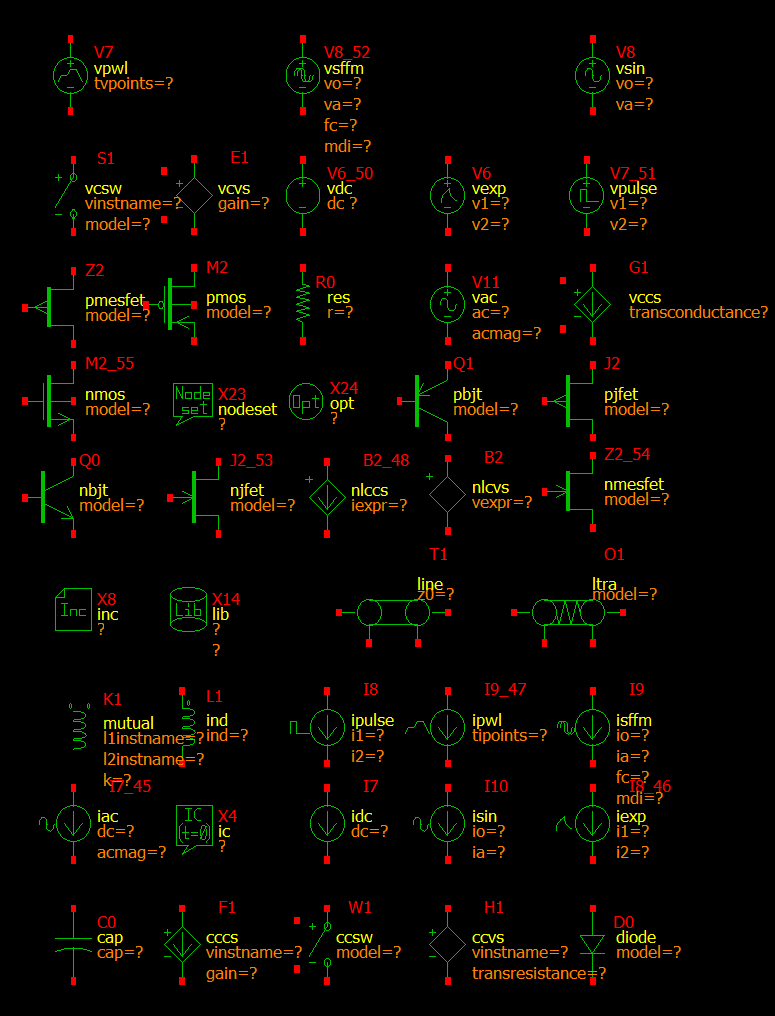
The library 'XyceLib' supplied with Glade contains device primitives (resistors, capacitors, MOS, bipolar, Jfet devices etc) for use in schematics you will simulate using Xyce or Spice.
You can use the Probe Window to set up probes for simulation plotting. A shortcut to entering nets to probe is to right click on them.
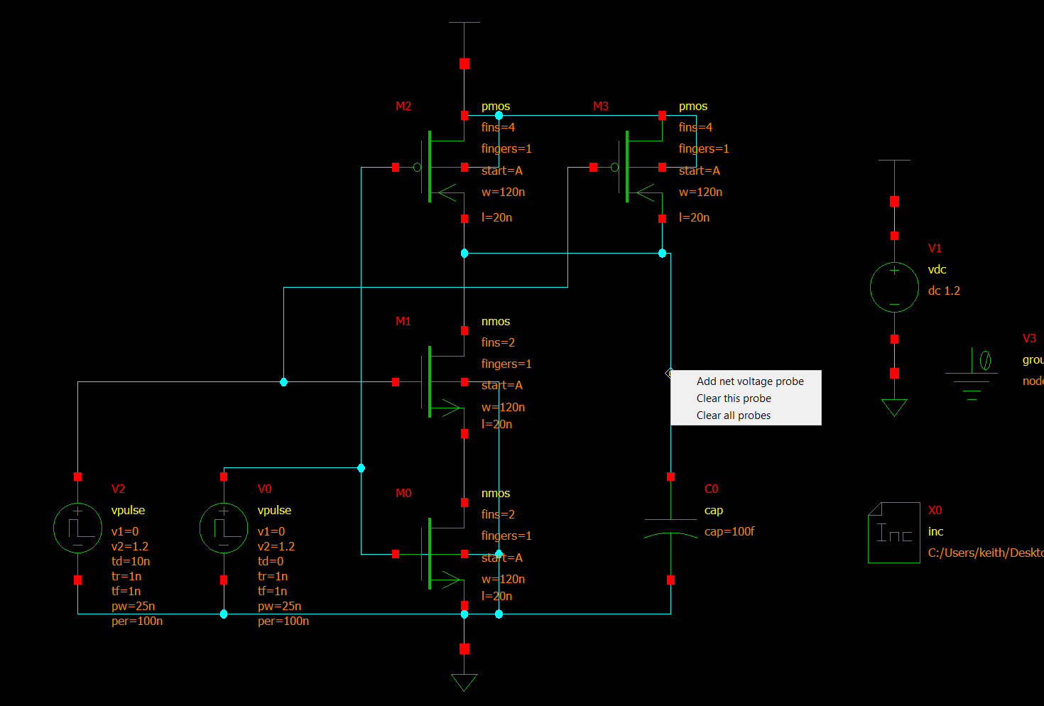
A popup menu appears when you right click on a net and allows you to add a voltage probe for that net, to clear an existing probed net or to clear all probed nets.
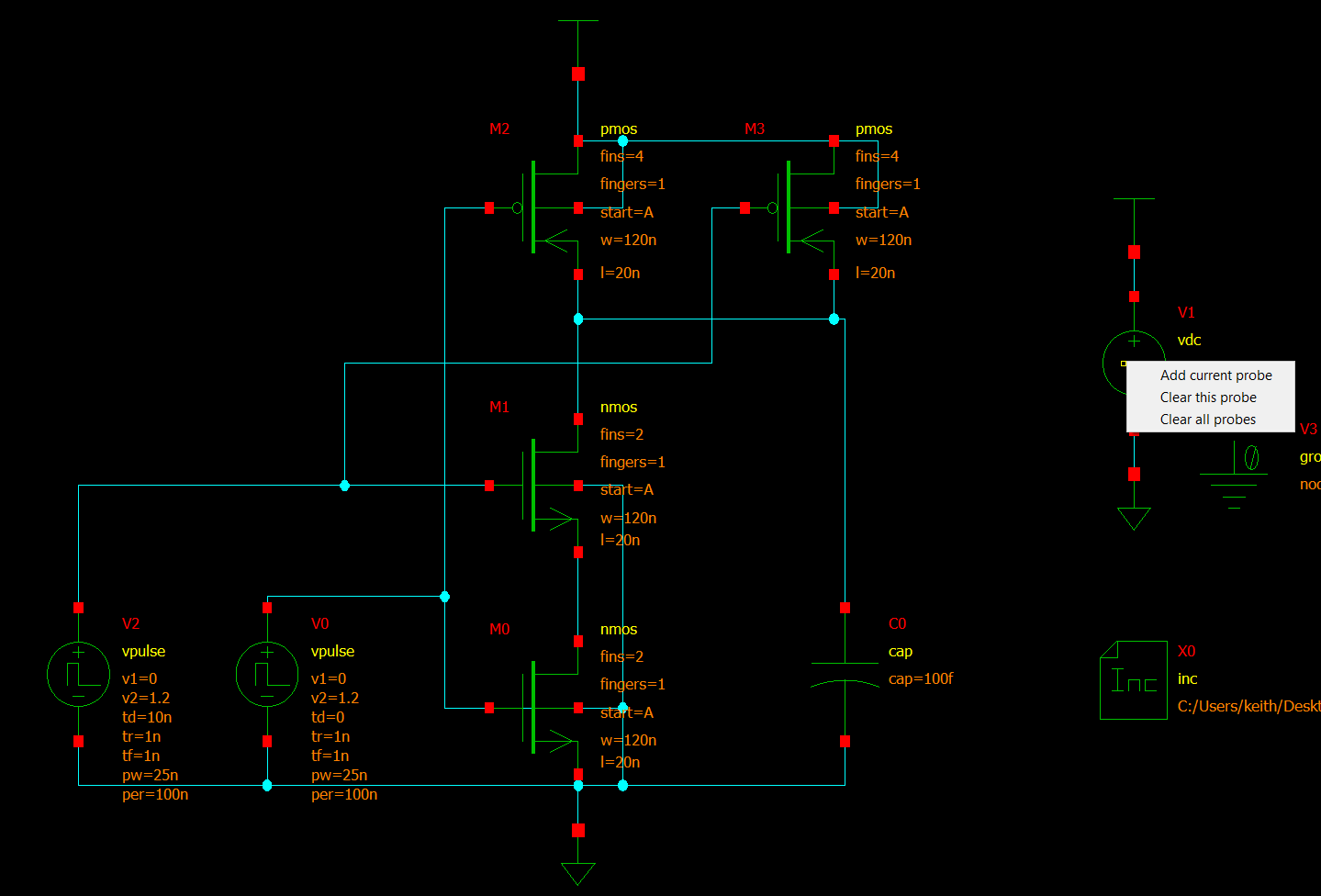
Similarly if you right click on a voltage source you can add a probe for its branch current:
Probes entered are shown in the probes window (Tools->Probe WIndow).
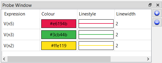
The first column of the probe window shows the expression passed to the simulator. So for probing the voltage on node n5, the probe expression is V(n5). Double left clicking on the expression allows you to edit it.
The second column shows the colour of the probe, as highlighted in the schematic, and shown in the plot window. The text is the colour in hex rgb format. Double clicking on the entry allows you to change the probe colour.
The third column shown the linestyle; double clicking again allows you to change this.
The fourth column shows the linewidth of the waveform in the plot window.
The + and - buttons allow you to add new probe expressions or delete existing ones manually. Note that probe expressions do not necessarily correspond to node names and can be anything the simulator supports.
The Simulation->Setup... menu sets the simulator runtime options and netlisting options.
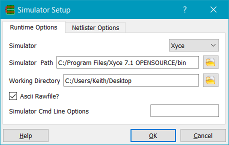
Simulator sets the simulator name. It is a cyclic field of suppported simulators. Simulator Path is the path to the simulator executable. The combination of simulator path and name is used to invoke the simulator. Working Directory is the directory where e.g. netlisting and plot (rawfile) files are generated. Glade reads Spice3-style rawfiles for plotting; if Ascii Rawfile? is checked, the rawfile will be written in ascii, else it will be binary. Simulator Cmd Line Options are passed to the simulator on invocation.
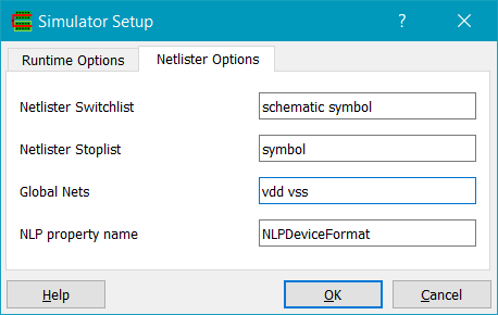
Netlister Switchlist is a whitespace delimited list of views that the netlister uses to switch into lower leves of a schematic hierarchy. Netlister Stoplist is a whitespace delimited list of views that the netlister will stop on and not descend further. Global Nets are nets which are added to the netlist as .GLOBAL, i.e. common throughout the subcircuit hierarchy. NLP Property Name is the name of the property that holds thenetlister formatting string.
To simulate a schematic only, the switchlist will normally be 'schematic symbol' and the stoplist 'symbol'. The netlister will then switch into schematic views in the hierarchy until it comes to a cell with a symbol view only; this will be output in the netlist, using it's NLPDeviceFormat property to set how the netlister writes the instance name, the nets connecting to the pins of the symbol instance etc.
If you want to simulate an extracted view e.g. the example lib 'opamp' cell, you need to set the switch list to e.g. 'extracted schematicsymbol' and the stop list to 'layout symbol'. In this case, if there is an extracted view found, the netlister will descend into that. The stoplist is set to 'layout symbol' as we want to stop on the layout views of the pcells.
You can set up different switch and stop lists for different operations and they will be saved to the gladerc.xml settings file.
The Simulation->Run DCOP Analysis command displays the dc operating point dialog.
If Backannotate To Schematic is checked, the DC operating point voltages are annotated to wires in the schematic as properties. They will be displayed if the wire is highlighted (set highlighting on in the Selection Options dialog).
The Simulation->Run Transient Analysis command displays the transient analysis dialog.
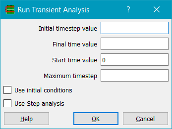
Initial timestep value is the minimum initial timestep used for simulation. Note that Xyce has slightly different meaning to this that e.g. Spice3; consult the Xyce user reference for details. Final Time Value is the simulation end time. Start Time Value is the time at which simulation results are stored; it is not the simulation starting time (which is always zero). Maximum Timestep is the maximum allowed timestep during simulation. Use Initial Conditions makes use of device initial conditions at the start of transient analysis. Use Step Analysis expands the form to allow a parameter to be stepped over a range, with a transient analysis for each value.
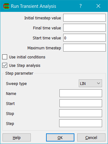
When Step Analysis is enabled, Sweep Type sets the type of the stepping - linear, decade or octave stepping. Name is the name of the parameter to be stepped, and Start, Stop and Step control the starting, stopping and step increment.
You can set up probes on nets before running transient analysis, and then the plot window will automatically be opened with the probed nets (or sources) displayed.
The Simulation->Run AC Analysis command displays the AC analysis dialog.
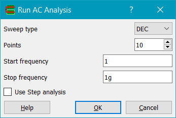
Sweep Type is the type of AC analysis; it can be Decade, Linear or Octave. Points is the number of analysis points per decade or octave, or the total number of points for a linear sweep. Start Frequency and Stop Frequency set the initial and final analysis frequencies. Use Step Analysis expands the form to allow a parameter to be stepped over a range, with an AC analysis for each value.
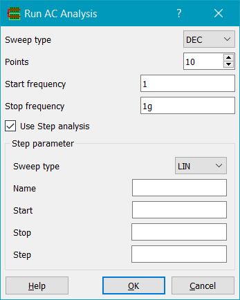
When Step Analysis is enabled, Sweep Type sets the type of the stepping - linear, decade or octave stepping. Name is the name of the parameter to be stepped, and Start, Stop and Step control the starting, stopping and step increment.
The Simulation->Run DC Analysis command displays the DC analysis dialog.
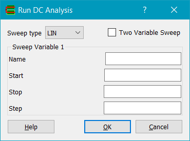
Sweep Type is the type of DC analysis for the sweep varable 1, and can be Linear, Decade, Octave or None. Name is the name of the first swept parameter. Start, Stop and Step set the starting, stopping and increment values. If Two Variable Sweep is set, a second swept variable can be used.
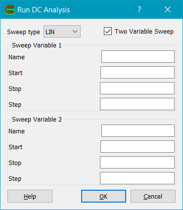
If Two Variable Sweep is checked,the second sweep variable name, start, stop and increment can be specified.
The Simulation->Plot... command displays the plot window..
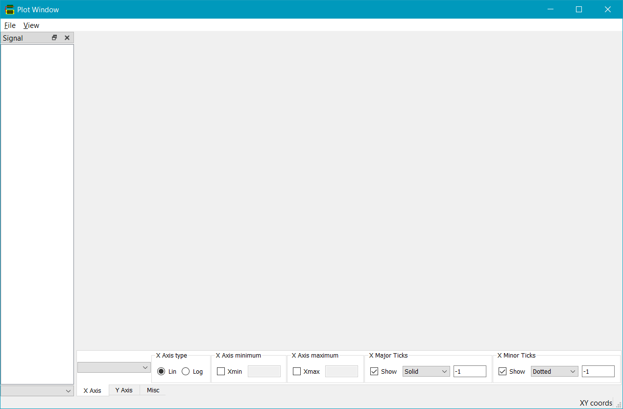
The plot window allows plotting node voltages, branchcurrents or expressions.
The plot window auto scales plotted expressions to the chart area.
The mouse wheel zooms in/out of the chart.
Clicking on a waveform with the left mouse button displays a callout (like a speech bubble) with the expression/variable name and X/Y values. You can have any number of callouts set, and they will be maintained on zooming or panning. Note that you must click precisely on the waveform to generate a callout.
Clicking with the right mouse button shows a popup menu that allows you to clear all callouts.
Right mouse button dragging zooms into a region of the chart. By default a rectangular area is zoomed into. Holding the Shift key while dragging zooms in by X axis only; holding the Ctrl key while dragging zooms in by Y axis only. Use View->Fit (f key) to reset the zoom.
The X axis and Y axis tabs allow chart X axis and Y axis to be controlled. The axis type can be Log or Linear. By default the axes are auto scaled; however checking e.g. Xmin or Xmax allows entering minimum/maximum limits for the axes. Major ticks and minor ticks are shown and automatically chosen; they can be manually shown/hidden;, their linestyles chose and the number of ticks set (-1 signifies use the default settings).
The Misc tab allows control over whether a single chart is used by all waveforms (the default), or a chart per waveform is 'Multiple Plots' is checked. Changing this option removes all plot expressions; they can be re-added by clicking on their names in the Signal dock window. Show Data Points shows the actual simulation data; else a spline fit to the data points is drawn.
Copyright © Peardrop Design 2026.