Glade Reference
Glade supports design rule checking and connectivity extraction using the Python scripting language to write DRC/extraction decks. The advantage of this is that you are using the same procedural language as the rest of the database and UI functionality. An example python DRC script looks like:
from ui import *

  # Get the open cellView

  cv = getEditCellView()

  geomBegin(cv)

  # Get layers

  active = geomGetShapes("active", "drawing")

  poly   = geomGetShapes("poly", "drawing")

  # Form derived layer

  gate   = geomAnd(active, poly)

  # Run width check

  geomWidth(gate, 0.18 "gate width < 0.18um")

  geomEnd()
In this example we first initialise the geometry package and tell it we want to check the current editing cellview with the geomBegin(cv) command. We then get shapes on different layers and perform boolean operations on them. Finally we check the derived layer using the geomWidth function. By default this writes DRC violations shapes to the TECH_DRCMARKER_LAYER (drcMarker layer in the LSW).
After completing DRC operations we call geomEnd() to free memory.
In the above example, 'active' and 'poly' are original layers. 'gate' is a derived layer that does not exist in the original cellView.
Before using DRC or LPE (extraction) commands, we normally need to perform some layer processing using boolean operations or select operations. For example in order to extract a MOS transistor, we need to identify the gate area by using the geomAnd() of the poly and diffusion layers, and we need to use the geomAndNot() of the diffusion and poly layers to split the diffusion between the source and the drain of the device, else we end up with all devices S/D terminals shorted.
The following layer processing functions are supported. Note that these don't have to be used just for DRC or LPE - you can use them in any python script for layer processing. The 'layers' that the commands produce are in fact temporary binary edge files. These files are called file0000.dat, file0001.dat etc. and are automatically deleted during geomEnd(). By default the layer files are written in the directory that Glade is invoked in. However if the environment variable GLADE_DRC_WORK_DIR is set to a valid directory, then they will be written to that directory instead.
Optional arguments are shown as e.g. hier=True, indicating that the default value of True is used if the argument is not specified.
Initialise the DRC package. A valid cellView must be passed to initialise the package. The cellView will be the one that subsequent processing operates on. Note the former equivalent function drcInit(cv) is still supported, but deprecated.
Uninitialise the DRC package. Working memory is freed. Temporary layer files are deleted. Note the former equivalent function drcUnInit(cv) is still supported, but deprecated.
Initialises out_layer with all shapes on the layer layerName, with purpose purpose. purpose defaults to 'drawing' if not given. The resulting derived out_layer contains merged shapes. The default is to get all shapes through the hierarchy; if the optional parameter hier is False, then only top level shapes are processed.
out_layer = geomStartPoly(vertices)
Creates a polygon from the given vertices list and saves to the layer out_layer, which will be overwritten if it exists. The resulting output layer is not merged. The vertex list must be in counterclockwise order and not self-intersecting. For example:
y4 = geomAddShape([ [0,0], [1000, 0], [1000, 2000], [0, 2000] ])
out_layer = geomAddPoly(layer, vertices)
Adds a polygon from the given vertices to the edge layer layer, and saves to the layer out_layer. The resulting output layer is merged with existing shapes on the layer. The vertex list must be in counterclockwise order and not self-intersecting. For example:
y3 = geomAddShapes(y3, [1000, 0], [1000, 2000], [0, 2000] ])
out_layer = geomAddShape(layer, shape)
Adds a shape shape to the edge layer layer. The resulting output layer is merged. For example:
y4 = geomEmpty()
cutshape = cv.dbCreateRect(cut, y4_lyr)
y4 = geomAddShape(y4, cutshape)
out_layer = geomAddShape(layer, shapes)
Adds a python list of shapes to the edge layer layer. The resulting output layer is merged. For example:
y3 = geomEmpty()
shapes = []
   for i in range(0,4) :
   shape = cv.dbCreateRect(box, y3_lyr)
   box.offset(2000, 0)
   shapes.append(shape)
y3 = geomAddShapes(y3, shapes)
Returns the number of shapes in a layer. This can be used as a test, e.g.
	if geomNumShapes(diff) != 0 :
		gate = geomAnd(poly, diff)
out_layer = geomEmpty()
Creates a dummy empty out_layer .
out_layer = geomBkgnd(size = 0.0)
Creates out_layer with an extent the size of the cellView's bounding box, plus size (which defaults to 0.0um). This is useful for example to create a pwell layer when the original mask data just has nwell information:
nwell = geomGetShapes('nwell', 'drawing')
bkgnd = geomBkgnd()
psub = geomAndNot(bkgnd, nwell)
geomErase('layerName', purpose='drawing')
Erases any design data on layer layerName in the current cellView. purpose defaults to 'drawing' if not given. Beware: there is no way of undoing this operation.
Returns the merged shapes on layer. This is equivalent to a single layer OR. Note that geomGetShapes() always merges raw input data, so there is normally no need to separately merge layers.
Returns the OR (union) of the two layers.
Returns the AND (intersection) of the two layers.
Returns the inverse of the layer. Effectively it runs geomAndNot(), with the first 'layer' being a rectangle the size of the cellView's bounding box, and the second the specified layer.
Returns the AND NOT of layer1 with layer2. This is equivalent to subtracting all shapes on layer2 from layer1.
out_layer = geomXor(layer1, layer2)
Returns the XOR of the two layers.
Sizes the layer by size microns. A positive size grows the layer, while a negative size shrinks the layer. If a shape should shrink so its width becomes zero, it will no longer be present in the sized_layer . The third argument, flag, if not specified sizes all edges by size. If flag is set to 'vertical' then sizing is only done in the vertical direction, if flag is set to 'horizontal' then sizing is only done in the horizontal direction.
Converts layer to trapezoids. If layer has connectivity established via geomConnect(), the connectivity will be maintained in the trapezoids generated.
Selection functions
Select all shapes on layer2 that touch layer1. Touching is defined as any edge of layer2 polygons that touch an edge from a layer1 polygon. flag can be layer1 or layer2 (the default), and controls which of the two layers that meet the criteria are output to touching_layer.
Select all shapes on layer2 that touch layer1. Overlapping is defined as any edge of layer2 polygons that intersects an edge from a layer1 polygon, i.e. the layer2 polygon is part inside, part outside layer1. flag can be layer1 or layer2 (the default), and controls which of the two layers that meet the criteria are output to overlapping_layer.
select_layer = geomInside(layer1, layer2, flag=layer2)
Select all shapes on layer2 that are inside (enclosed by) layer1. Shapes are considered as 'inside' if the shapes have common area. The layer2 edges may be coincident with layer1 edges. flag can be layer1 or layer2 (the default), and controls which of the two layers that meet the criteria are output to inside_layer.
select_layer = geomContains(layer1, layer2, flag=layer2)
Select all shapes on layer2 that are contained by shapes on layer1. Shapes are considered as 'contained' if all of their vertices are inside layer1 and do not touch layer1. flag can be layer1 or layer2 (the default), and controls which of the two layers that meet the criteria are output to contains_layer.
select_layer = geomOutside(layer1, layer2, flag=layer2)
Select all shapes on layer2 that are outside layer1. The shapes may touch or abut layer1. To make sure that shapes on layer2 are completely 'outside' layer1, and get considered, the 'enclosing' shape should be layer1. flag can be layer1 or layer2 (the default), and controls which of the two layers that meet the criteria are output to outside_layer.
select_layer = geomAvoiding(layer1, layer2, flag=layer2)
Select all shapes on layer2 that avoid layer1 and do not touch or overlap. flag can be layer1 or layer2 (the default), and controls which of the two layers that meet the criteria are output to avoiding_layer.
select_layer = geomButting(layer1, layer2, flag=layer2)
Select all shapes on layer2 that have outside edges that abut layer1 outside edges. flag can be layer1 or layer2 (the default), and controls which of the two layers that meet the criteria are output to butting_layer.
select_layer = geomCoincident(layer1, layer2, flag=layer2)
Select all shapes on layer2 that have edges coincident with inside edges of layer1. flag can be layer1 or layer2 (the default), and controls which of the two layers that meet the criteria are output to coincident_layer.
select_layer = geomInteracts(layer1, layer2, flag=layer2)
Select shapes on layer2 that interact with shapes on layer1. An interaction is defined as overlapping, abutting, coincident, or inside. flag can be layer1 or layer2 (the default), and controls which of the two layers that meet the criteria are output to interacting_layer.
Gets all shapes on layer that have text labels on the layer/purpose pair given by layerName / purpose. purpose defaults to drawing if not given. Optionally a name can be supplied e.g. 'vdd', and then only shapes with text labels with that name are output to out_layer .
Gets all shapes on layer1’s layer (which must be an input or derived layer specified in geomConnect) that are assigned to net with name ‘netName’.
out_layer = geomHoles(layer)
Gets the holes in polygons on layer and outputs them to out_layer.
out_layer = geomNoHoles(layer)
Gets the polygons on layer and outputs them, minus any holes, to out_layer.
out_layer = geomGetHoles(layer, flag=greaterthan, count=0)
Gets the holes on layer polygons and outputs them, to out_layer. flag and count set the criteria; for example greaterthan, 1 will only output holes for polygons which have more than 1 hole.
out_layer = geomGetHoled(layer, flag=greaterthan, count=0)
Gets the polygons on layer that do not contain holes and outputs them, to out_layer. flag and count set the criteria; for example equals, 2 will output original polygons (less their holes) for polygons with exactly 2 holes.
out_layer = geomGetNon90(layer)
Gets the polygons on layer and outputs ones that have one or more edges that are non 90 degrees to out_layer.
out_layer = geomGetNon45(layer)
Gets the polygons on layer and outputs ones that have one or more edges that are non 90 and non 45 degrees to out_layer
out_layer = geomGetRectangles(layer)
Gets the shapes on layer and outputs ones that are rectangular, i.e. have 4 edges parallel to the X or Y axes.
out_layer = geomGetPolygons(layer)
Gets the shapes on layer and outputs ones that are not rectangular, i.e. have at least one edge not parallel to the X or Y axes.
out_layer = geomGetVertices(layer1, num, flags = equal)
Get shapes on layer1’s layer that have num vertices. Optionally flags can be set to equal, not_equal, greater, less.
DRC functions, like boolean operations, are edge-based, using a Bentley-Ottman scanline algorithm. Edges are currently only considered in error if they project onto each other in the X or Y direction and the spacing between the edges is less than the specified rule. Perpendicular edges are not considered errors. The resulting error marker shapes are constructed from the four vertices of the error edges, and are copied to the output layer where they may be used for subsequent boolean operations.
Many commands take a flags parameter. Flags can be bitwise OR's together using the '|' operator, although some flags are mutually independent: samenet/diffnet; equals/not_equal/greaterthan, greaterorequal, lessthan, lessorequal; horizontal/vertical/diagonal; layer1/layer2; butting/coincident/inside/outside/over/not_over.
The flags are:
Single layer width check. Checks layer for minimum width violations i.e. widths less than rule. Error polygons are created on the drcMarker layer in the current cellView. The rule dimension must be specified in microns.
An optional message will be written as a property 'drcWhy' on the marker shape if specified.
Checks layer for minimum width violations i.e. widths less than rule. Error polygons are created on the drcMarker layer in the current cellView. The rule dimension must be specified in microns.
Allowable flags are:
An optional message will be written as a property 'drcWhy' on the marker shape if specified.
Checks layer for width violations. The widths must be discrete values specified in rules, which is a python sequence. Error polygons are created on the drcMarker layer in the current cellView. The rules must be specified in microns.
Allowable flags are:
An optional message will be written as a property 'drcWhy' on the marker shape if specified.
Example:
geomAllowedWidths(poly, [0.020, 0.022, 0.024], horizontal)
Checks layer1 for edge length violations i.e. lengths less than rule, where edges of layer1 related to shapes on layer2 are checked. The relation of layer1 edges to layer2 edges can be specified by flags. Possible checks are:
Error polygons are created on the drcMarker layer in the current cellView. The rule dimension must be specified in microns.
Allowable flags are:
An optional message will be written as a property 'drcWhy' on the marker shape if specified.
Example:
geomEdgeLength(gate, active, 0.13, coincident, "Gate length < 0.13um")
Checks layer for minimum spacing violations i.e. single layer spacings less than rule. Error polygons are created on the drcMarker layer in the current cellView. The rule dimension must be specified in microns. Note that spacing violations between edges of the same polygon are not reported; to detect these perform a geomNotch check. An optional message will be written to the error marker flag if specified. flags can be used to control the spacing check. A flag of samenet applies the check only if the two shapes are on the same physical net. flags can be used to control the spacing check.
Allowable flags are:
Example:
geomSpace(active, 0.2, samenet, "active space < 0.2 for same net")geomSpace(active, 0.3, diffnet, "active space < 0.3 for different nets")
Checks layer for minimum spacing violations i.e. single layer spacing less than rule, where one of the shapes has a width > width and a parallel run length > length. Error polygons are created on the drcMarker layer in the current cellView. The rule and width dimensions must be specified in microns. Note that spacing violations between edges of the same polygon are not reported; to detect these perform a geomNotch check. An optional message will be written to the error marker flag if specified. flags can be used to control the spacing check.
Allowable flags are:
Example:
geomSpace(active, 0.2, 10.0, samenet, "active space < 0.2 for same net with width > 10.0")
geomSpace(active, 0.3, 10.0, diffnet, "active space < 0.3 for different nets with width > 10.0")
Checks layer for minimum spacing violations i.e. single layer spacing less than rule, where both of the shapes has a width > width and a parallel run length > length. Error polygons are created on the drcMarker layer in the current cellView. The rule and width dimensions must be specified in microns. Note that spacing violations between edges of the same polygon are not reported; to detect these perform a geomNotch check. An optional message will be written to the error marker flag if specified. flags can be used to control the spacing check.
Allowable flags are:
Example:
geomSpace2(active, 0.2, 10.0, samenet, "active space < 0.2 for same net with width > 10.0")geomSpace2(active, 0.3, 10.0, diffnet, "active space < 0.3 for different nets with width > 10.0")
Checks layer1 to layer2 for minimum spacing violations i.e. two layer spacings less than rule. Error polygons are created on the drcMarker layer in the current cellView. The rule dimension must be specified in microns. An optional message will be written to the error marker flag if specified. flags can be used to control the spacing check.
Allowable flags are:
Example:
geomSpace(nwell, ndiff, 0.2, samenet, "nwell to n+ diff space < 0.2 for same net")
geomSpace(nwell, ndiff, 0.3, diffnet, "nwell to n+ diff space < 0.3 for different nets")
Single layer length dependent spacing check. Checks layer1 for minimum spacing violations i.e. single layer spacing less than rule, where the shapes have a parallel run length that can be lessthan, greaterthan, equals not not_equal to length, according to flags. Error polygons are created on the drcMarker layer in the current cellView. The rule and length dimensions must be specified in microns as a float. Note that spacing violations between edges of the same polygon are not reported; to detect these perform a geomNotch check. An optional message will be written to the error marker flag if specified. flags can be used to control the runlength check.
Allowable flags are:
Example:
geomSpace(active, 0.2, 10.0, lessthan, "active space < 0.2 with runlength < 10.0")
Checks layer for space violations. The spaces must be discrete values specified in rules, which is a python sequence. Spacing greater or equal to the last rule is allowed. Error polygons are created on the drcMarker layer in the current cellView. The rules must be specified in microns.
Allowable flags are:
An optional message will be written as a property 'drcWhy' on the marker shape if specified.
Example:
geomAllowedSpaces(active, [0.020, 0.022, 0.024], horizontal)
In the above, the layer 'active' must have spacing of either 20nm, 22nm or >= 24nm.
out_layer = geom2DSpace(layer, rules, flags, message=None)
Checkes layer for spacing that is both length and width dependent. The rules consist of a 2D python array, of which row 0 defines the widths of the rules, and column 0 defines the lengths of the rules. The other entries are the rule values. flags are as defined above. An optional message will be written as a property 'drcWhy' on the marker shape if specified.
Example:
 geom2DSpace(m1,  [ [0.000, 0.028, 0.032, 0.040, 0.064, 0.120, 0.240, 0.320, 0.600],
 [0.028, 0.036, 0.036, 0.036, 0.036, 0.036, 0.036, 0.036, 0.036],
 [0.240, 0.036, 0.068, 0.076, 0.076, 0.076, 0.076, 0.076, 0.076],
 [0.480, 0.036, 0.068, 0.076, 0.092, 0.092, 0.092, 0.092, 0.092],
 [1.200, 0.036, 0.068, 0.076, 0.092, 0.120, 0.120, 0.120, 0.120],
 [1.800, 0.036, 0.068, 0.076, 0.092, 0.120, 0.240, 0.240, 0.240],
 [2.400, 0.036, 0.068, 0.076, 0.092, 0.120, 0.240, 0.320, 0.600]
 ], 0, "M1 Minimum spacing")
The above defines a minimum rule of 28nm for normal metal. For metal wider than 240nm then if the width is wider than 32nm the rule is 68nm, if the width is wider than 40nm the rule is 76nm etc.
Single layer nearest neighbour check. Checks layer1 shapes for neighbouring shapes within dist. If there are more than num shapes within rule, then an error is generated. This check is for contacts/vias in e.g. 40nm or below processes; only rectangular shapes can be checked.
Allowable flags are:
Example:
   geomNeighbours(CO, 0.11, 0.10, 3,  "CO Space to 3 neighbours < 0.10 (CO.S.2)")
   The above checks if there are 3 neighbouring CO shapes  within 0.11um of a CO shape. If so they have to be spaced by 0.10um.
Checks layer1 polygons for notch violations. Error polygons are created on the drcMarker layer in the current cellView. The rule dimension must be specified in microns. Note that notches are effectively spacing violations between edges of the same polygon. An optional message will be written as a property 'drcWhy' on the marker shape if specified.
Allowable flags are:
Checks layer1 for minimum line end spacings. The spacing is from the line end edge to another edge which is either a normal edge (if num_ends=1) or another line end edge (if num_ends = 2). A line end edge is a horizontal edge with two adjacent vertical edges, or a vertical edge with two adjacent horizontal edges. The adjacent edge length must be greater than the line end edge length, or min_adj_edge_length, whichever is the greater. The rule dimension and the min_adj_edge must be specified in microns.
Allowable flags are:
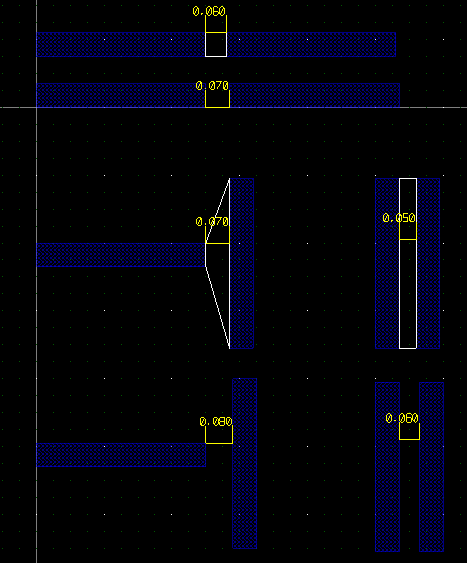
In the above example, the rules are as follows:
geomSpace(metal1, 0.06)
geomLineEnd(metal1, 0.08, 1)
geomLineEnd(metal1, 0.07, 2)
As above but for two layer checking.
Checks that layer1 is on a pitch greater than or equal to the rule specified. flags can be vertical or horizontal. An optional message will be written as a property 'drcWhy' on the marker shape if specified.
Allowable flags are:
Checks layer1 to layer2 for minimum overlap violations i.e. layer1 overlaps layer2 by less than rule. Error polygons are created on the drcMarker layer in the current cellView. The rule dimension must be specified in microns. An optional message will be written as a property 'drcWhy' on the marker shape if specified.
Allowable flags are:
Checks layer1 to layer2 for minimum enclosure violations i.e. layer1 encloses layer2 by less than rule. Error polygons are created on the drcMarker layer in the current cellView. The rule dimension must be specified in microns. The optional flags can have the 'abut' flag set which considers abutting edges an error; otherwise abutting edges are allowed. An optional message will be written as a property 'drcWhy' on the marker shape if specified.
Allowable flags are:
Checks layer1 to layer2 for minimum enclosure violations. layer1 should enclose layer2 by rule1 normally. However if there 1 or more edges of layer2 with enclosure greater than or equal to rule2, but less than rule1, and edges (e.g. 2) perpendicular edges of layer1 enclose layer2 by greater than or equal to rule3, then no violation occurs. The rule* dimensions must be specified in microns. An optional message will be written to the error marker flag if specified. Any edge enclosure less than rule2 will give an error. The parameter edges must be 1 or 2.
Example:
geomEnclose2(nwell, active, 0.18, 0.08, 0.23, 2)
Enclosure of active by nwell should be >= 0.18um, however if 2 parallel edges of active have a nwell enclosure of 0.08um then the other two perpendicular edges should have a minimum enclosure of 0.23um.
geomEnclose2(cont, metal, 0.15, 0.05, 0.30, 1)
Enclosure of cont by metal should be 0.15um, however an edge can be enclosed by 0.05um if one perpendicular edge is greater than or equal to 0.3um.
Checks layer1 to layer2 for minimum enclosure violations. layer1 must enclose layer2 according to rules, which is a list of triplets e.g. [ [0.010, 0.010, 4], [0.0, 0.032, 2], [0.002, 0.028, 2] ]. For each triplet, the first two numbers are allowed enclosures, and the third number is the number of sides that must obey the second rule. For example, in the first case [0.010, 0.010, 4] all 4 sides of layer2 can be enclosed by 10nm. In the second case [0.0, 0.032, 2] there can be 2 opposite sides with enclosure of 0nm, and the other two sides must have an enclosure of 32nm. Finally in the third case [0.002, 0.028, 2] there can be 2 opposite sides with enclosure of 2nm and the other two sides must have enclosure of 28nm. These are the only allowed enclosure values; anything else will give a violation. The rule dimensions must be specified in microns. An optional message will be written as a property 'drcWhy' on the marker shape if specified.
Checks layer1 to layer2 for minimum extension violations i.e. layer1 extends beyond layer2 by less than rule. Error polygons are created on the drcMarker layer in the current cellView. The rule dimension must be specified in microns. An optional message will be written as a property 'drcWhy' on the marker shape if specified.
Allowable flags are:
Checks layer1 shapes for minimum area violations that meet the condition (minrule < area) || (area < maxrule). Error polygons are created on the drcMarker layer in the current cellView. The minrule and optional maxrule dimensions must be specified in microns. An optional message will be written as a property 'drcWhy' on the marker shape if specified.
Single layer area check. Checks layer1 shapes for minimum area violations that meet the condition minrule op area. Error polygons are created on the drcMarker layer in the current cellView. The minrule dimension must be specified in microns as a float. An optional message will be written as a property 'drcWhy' on the marker shape if specified.
Allowable flags to control op are:
Checks layer1 shapes and flags shapes that meet the condition (area > minrule) && (area < maxrule). Error polygons are created on the drcMarker layer in the current cellView. The minrule and optional maxrule dimensions must be specified in microns. An optional message will be written as a property 'drcWhy' on the marker shape if specified.
Single layer internal (hole) area check. Checks layer1 shapes and flags shapes that meet the condition area op minrule. Error polygons are created on the drcMarker layer in the current cellView. The minrule and optional maxrule dimensions must be specified in microns as a float. An optional message will be written as a property 'drcWhy' on the marker shape if specified.
Allowable flags to control op are:
Checks layer1 for minimum density of the layer, where rule is the percentage of the layer area of the design bounding box. An optional message will be written as a property 'drcWhy' on the marker shape if specified. This function returns the area in square dbu of the layer.
Checks layer1 for maximum density of the layer, where rule is the percentage of the layer area of the design bounding box. An optional message will be written as a property 'drcWhy' on the marker shape if specified. This function returns the area in square dbu of the layer.
Checks layer1 for density locally in a rectangle of size given by window_x and window_y. The window is stepped in increments of step_x and step_y over the design bounding box. Flags will determine how the area rule is applied (rule is a percentage). An optional message will be written as a property 'drcWhy' on the marker shape if specified.
Allowable flags are:
Checks layer1 shapes for minimum margin violations. A margin violation is the distance (typically greater than the normal minimum spacing), from the vertex common to two adjacent concave edges of a polygon, to edge(s) of a nearby polygon. Error polygons are created on the drcMarker layer in the current cellView. The rule dimension must be specified in microns. An optional message will be written as a property 'drcWhy' on the marker shape if specified.
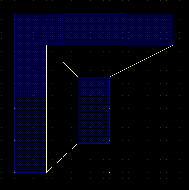
In the above example, the distance of the inner (concave) edge of the L shaped polygon vertex is less than the specified rule to the nearest vertex of the rectangle. Two error flags are created because there are two edges of the rectangle containing the vertex in violation.
Checks all layer1 vertices of edges to see if they are on a multiple of the grid specified in microns by grid. marker_size is the size of the marker in microns (shown as a '+' centered on the offgrid vertex) on the drcMarker layer. An optional message will be written to the error marker flag if specified. The return value is the number of off-grid vertices found.
Checks vertices for adjacent edge length, If one edge has length less than length, the other edge must have length greater than rule.An optional message will be written as a property 'drcWhy' on the marker shape if specified.
Allowable flags are:
Checks the size of rectangular shapes e.g. contacts or vias. rule specifies the permissible edge lengths as length/width pairs.An optional message will be written as a property 'drcWhy' on the marker shape if specified.
For example:
geomAllowedSize(via, [[0.028, 0.028],[0.028,0.056]], "Via is rectangular 28x28 or 28x56nm")
Checks shapes on the layer via which must be rectangles with either sides of 28nm or 2 sides of 28nm and 2 sides of 56nm.
Returns the number of errors detected in the most recent DRC check.
Returns the total number of DRC errors since the start of the run.
Extraction
Glade can trace connectivity in a layout and identify devices such as resistors, capacitors, diodes, mos and bipolar transistors plus parasitic capacitors. To extract a layout, a python script is used to form derived layers, run connectivity tracing and extract devices. The results are saved to a cellView with the viewName of ‘extracted’ but this can be changed using the setExtViewName command.
Extraction rules consist of 4 steps:
Derived layers are used to identify devices and break connecting layers such as poly or diffusion where they touch active devices.
A MOS device is formed by diffusion and poly layers. Two derived layers are generated; the recognition region, formed by using geomAnd() to produce the intersection of the tow layers, and the S/D terminals, produced by using geomAndNot() to subtract the poly area from the diffusion. This is necessary, else connectivity tracing on the diffusion would see a short between the S and D terminals. Connectivity tracing is performed using the geomConnect command. This traces connectivity through specified layer-layer overlaps, for example metal1 connectivity to poly though a contact layer. Device extraction is performed using the extract… commands. When devices are extracted, an extraction PCell (e.g. nch_ex.py in the example data) is used to form an instance in the extracted view which is connected via the layers traced in geomConnect. The PCell is passed the coordinates of the recognition region used to identify the device, along with any properties for the particular type of device. Saving interconnect is done using the saveInterconnect() function. This takes a derived layer and maps it back to a technology file layer/purpose. The layers being saved should have been present in a geomConnect() command previously. Parasitic extraction determines capacitance between connect layers either using a simple area/perimeter calculation, or a more accurate (but much slower) 3D field solver ‘Fastcap’.
The extracted view can be netlisted to a CDL/Spice file; there are two methods by which the netlister will format the lines for each instance in the file. If a string property named ‘NLPDeviceFormat’ is present on the PCell master, this property allows user defined netlisting. See ‘NLP expressions’ for more details of the NLPDeviceFormat syntax. If this property is not present, the netlister will look for hardcoded property names on devices:
The hardcoded netlister expects specific pin names on the extraction PCell devices:
Sets the name of the extracted view. The default is "extracted", but for e.g. abstract generation you can set this to "abstract". Note this command should be given before any saveDerived / saveInterconnect commands.
Trace connectivity through layers. This function takes a list of lists of layers, where the layers are a via or contact layer and the layers that are connected by it. For example:
geomConnect( [
    [cont, active, poly, metal1],
    [via1, metal1, metal2]
] )
The above will connect active and metal1 by the cont layer, poly and metal1 also by the cont layer, and metal1 and metal2 by the via1 layer. There is no limit to the number of lists of layers, or to the number of layers connected by a contact layer. However the list of connected layers must have only one contact/via layer, and that layer must be the first layer in the list. If shapes already have net information (e.g. through the use of the geomLabel() command) then these shapes are used as initial tracing points, and net names are propagated to connected shapes. Other shapes are assigned automatically generated names (n0, n1, n2 etc). Shorts between shapes with assigned or traced net names that are different are reported.
The geomConnect() command is multithreaded in version 4.3.21 and beyond. This can be controlled by setting the environment variable GLADE_THREADED_EXTRACTION. The env var can take an optional value, being the maximum number of threads to run. For example on a Core i7 cpu with 4 physical cores each capable of running 2 threads, you could set GLADE_THREADED_EXTRACTION=8
.
Label a layer with existing text labels. If a text label with layer layerName and purpose purpose has its origin contained in a shape on layer, then the shape will have its net name set to the text label name. Note that labelling layers should be performed prior to connectivity extraction for net name propagation. Logical nets/pins will be created in the extracted view for all text labels that attach to shapes on layer. If not specified, labelPurpose defaults to "drawing" . Note that labels are only used for the top level of the design; in other words labels at lower levels of the layout hierarchy are ignored. For LVS purposes, labelling power, ground, clock and primary IOs is all that is usually necessary. createPin can be set to False (default is True) to disable creating a pin - only a net will be created.
ok = geomSetText(layer, xcoord, ycoord, 'labelName', createPin = True)
Labels layer with text label labelName at the coordinates given by xcoord and ycoord (in microns). Returns True if a shape on the layer was found at the given xy coordinates; False if no shape was found (i.e. the command failed). This is useful if you cannot modify the original layout and want to try and resolve LVS errors by forcing a shape to be a specified net name. createPin can be set to False (default is True) to disable creating a pin - only a net will be created.
Outputs layer geometries as polygons to the current cellView. The layer they are output to can be set by outLayer, which defaults to the drcMarker layer. Each polygon has a string property drcWhy with value set to the string why.
Outputs layer geometries as polygons to the current cellView. The layer they are output to can be set by layerName and purpose. If viewType is specified, the layer geometries are output to this view name rather than the default view name 'extracted'.
Creates a new cellview with the same cell name as the current cell, and a view name of 'extracted'. Shapes on layers specified are created in the extracted cellview. Shapes will have net information if they are on layers present in geomLabel and/or geomConnect() commands. Optionally instead of a layer name, a list of derived layer name, a techfile layer name and optionally a purpose can be specified, for example:
saveInterconnect( [
	   poly,
	   active,
	   [ metal1, 'M1' ],
	   [ metal2, 'M2', 'pin']
] )
Original layers that are generated from geomGetShapes() do not need the techfile layer name/purpose specified, but derived layers MUST specify the target layer name, else they will be assigned a fake layer number which the LSW will not show. It is often desirable to add dummy layers to the techfile and use these for saveInterconnect(). For example, when extracting a lateral PNP, derived layers for emitter, base and collector need to be generated for the extractBjt() terminals. In this case it's desirable to have dummy layers 'emitter', 'base' and 'collector' so that devices get extracted correctly.
If an existing layer name is specified without a purpose name, the purpose name defaults to 'drawing'. There is no limit on the number of layers in the list. Note that any terminal layer used in subsequent 'extract...' commands should be saved.
Extracts MOS devices and creates instances of a cellView 'modelName layout' in the extracted view. recLayer is the recognition layer of the gate region. gateLayer is the poly layer and diffLayer is the source/drain diffusion layer. bulkLayer is the optional well layer; if present the extracted instances have terminals D G S B, otherwise 3 terminal devices with terminals D G S are extracted. The layers gateLayer, diffLayer and bulkLayer must have previously been saved using the saveInterconnect command.
The extracted instances have the property 'w' set to the recLayer shape width (length of gate recognition shape edge coincident with diffLayer) and 'l' set to the distance between the coincident diffLayer/gateLayer edges. Both manhattan and any-angle gates are supported. The recLayer shapes should be a simple polygon without holes.
The cellview 'modelName layout' will be created if it does not already exist. If it does exist, it is assumed to be a PCell, and its ptlist property is set to the point list of the recognition region. Example nmos/pmos cells with parameterised point lists are nmos_ex.py and pmos_ex.py.
As above but allows the terminal names of the gate, source, drain and bulk terminals to be specified.
extractRes('modelName', recLayer, termLayer, bulkLayer=None)
Extracts a 2 terminal resistor and creates instances of a cellView 'modelName layout' in the extracted view. recLayer is the recognition layer for the resistor. termLayer is the layer of the resistor terminals e.g. poly, and shapes on this layer should overlap or touch the recognition layer shape. The layer termLayer must have previously been saved using the saveInterconnect command. If the optional layer bulkLayer is specified, an additional bulk node is generated for the resistor model.
The extracted instances will have the properties w set the the recLayer width (length of recLayer edge coincident with termLayer edge) and l set to the recLayer length (total length of all recLayer edges minus twice the width, then divided by two), nsquares set to l/w, nbends to the number of bends. These properties can be accessed via an extraction PCell - see the example 'pres_ex.py' in the distribution.
The cellview 'modelName layout' will be created if it does not already exist. If it does exist, it is assumed to be a PCell, and its ptlist property is set to the point list of the recognition region. If a PCell is used, its terminals are expected to be "A" and "B".
As above but allows the terminal names of the term layer and bulk layer(if used) to be specified.
extractMosCap('modelName', recLayer, gateLayer, diffLayer, bulkLayer=None)
Extracts a 2 terminal capacitor and creates instances of a cellView 'modelName layout' in the extracted view. recLayer is the recognition layer for the capacitor. gateLayer and diffLayer form the terminal layers of the capacitor, and these layers must have previously been saved using the saveInterconnect command.
The extracted instances will have the properties area set the the recLayer area and perim set to the recLayer perimeter.
The cellview 'modelName layout' will be created if it does not already exist. If it does exist, it is assumed to be a PCell, and its ptlist property is set to the point list of the recognition region. If a PCell is used, its terminals are expected to be "G" for the gate layer and "S" for the diff layer.
As above but allows the terminal names of the gate, S/D and optional bulk layer to be specified.
Extracts a 2 terminal diode and creates instances of a cellView 'modelName' layout in the extracted view. recLayer is the recognition layer for the capacitor. anodeLayer and cathodeLayer form the terminal layers of the diode, and shapes on these layers should overlap or touch the recognition layer shape, and these layers must have previously been saved using the saveInterconnect command. .
The extracted instances will have the properties area set the the recLayer area and pj set to the recLayer perimeter.
The cellview 'modelName layout' will be created if it does not already exist. If it does exist, it is assumed to be a PCell, and its ptlist property is set to the point list of the recognition region. If a PCell is used, its terminals are expected to be "A" for the anode and "C" for the cathode.
As above but allows the terminal names of the anode, cathode and optional bulk layer to be specified.
Extracts a 3 terminal bjt and creates instances of a cellView 'modelName layout in the extracted view. recLayer is the recognition layer for the bjt. emitLayer, baseLayer and collLayer form the terminal layers of the bjt, and shapes on these layers should overlap or touch the recognition layer shape, and these layers must have previously been saved using the saveInterconnect command. .
The extracted instances will have the properties area set the the emitter recLayer area and perim set to the recLayer perimeter.
The cellview 'modelName layout' will be created if it does not already exist. If it does exist, it is assumed to be a PCell, and its ptlist property is set to the point list of the recognition region. If a PCell is used, its terminals are expected to be "C" for the collector, "B" for the base and "E" for the emitter.
As above but allows the terminal names of the emitter, base, collector and optional bulk layer to be specified.
Extracts TFT (thin film) MOS devices and creates instances of a cellView 'modelName layout' in the extracted view. recLayer is the recognition layer of the gate region. gateLayer is the poly layer and diffLayer is the source/drain diffusion layer. The layers gateLayer and diffLayer must have previously been saved using the saveInterconnect command. The gateLayer is normally the bottom metal1 plate and the diffLayer the top metal2 fingers.
The extracted instances have the property w set to the recLayer shape width (length of gate recognition shape coincident with diffLayer) and l set to the distance between the coincident edges. Both manhattan and any-angle gates are supported. The recLayer shapes should be simple polygons without holes.
The cellview 'modelName layout' will be created if it does not already exist. If it does exist, it is assumed to be a PCell, and its ptlist property is set to the point list of the recognition region. If a PCell is used, its terminals are expected to be "D" for the drain, "S" for the source and "G" for the gate.
Extracts a generic deviceand creates instances of a cellView 'modelName layout' in the extracted view. The first letter of the modelName should correspond to the Spice device type e.g. R for a resistor, C for a capacitor (case insensitive) etc. recLayer is the device recognition layer. The termLayer(s) should be connection layers previously saved by the saveInterconnect command. Each terminal layer can have one of more terminal names. Shapes on the terminal layer(s) that touch or overlap the recognition layer will be created as terminals of the device. The recLayer shapes should be a simple polygon without holes.
The cellview 'modelName layout' will be created if it does not already exist. If it does exist, it is assumed to be a PCell, and its ptlist property is set to the point list of the recognition region.
extractParasitic(metLayer, areaCap, perimCap, 'gndNetName')
Extracts the parasitic capacitance of net shapes on layer metLayer. metLayer can be any layer in the geomConnect() set of layers; for each (merged) shape on metLayer its area (in microns^2) and perimeter (in microns) are calculated and multiplied by the values of areaCap and perimCap. An instance of a capacitor is created (of size 100x100 database units so not normally visible) on one of the vertices of the shape, with property 'c' set to the area * areaCap + perimeter * perimCap. The capacitance will be connected to the shape's net and to the ground net specified by gndNetName.
extractParasitic2(metLayer1, met2Layer, areaCap, perimCap)
Extracts the parasitic capacitance of net shapes between layers met1Layer and met2Layer. The two layers can be any layer in the geomConnect() set of layers; for each intersection of met1Layer and met2Layer the area (in microns^2) and perimeter (in microns) are calculated and multiplied by the values of areaCap and perimCap. An instance of a capacitor is created (of size 100x100 database units so not normally visible) on one of the vertices of the shape, with property 'c' set to the area * areaCap + perimeter * perimCap. The capacitance will be connected between the nets of the shapes of each metal layer.
extractParasitic3(metLayer1, met2Layer, areaCap, perimCap, [layer1,...layerN])
Only extracts capacitance between metal1Layer and metal2Layer if shield layer(s) layer1... layerN are not present between them. Note no checkinig is done for valid layers (yet). The two layers can be any layer in the geomConnect() set of layers; for each intersection of met1Layer and met2Layer the area (in microns^2) and perimeter (in microns) are calculated and multiplied by the values of areaCap and perimCap. An instance of a capacitor is created (of size 100x100 database units so not normally visible) on one of the vertices of the shape, with property 'c' set to the area * areaCap + perimeter * perimCap. The capacitance will be connected between the nets of the shapes of each metal layer.
extractParasitic3D('subsNetName', 'refNetName', tol=0.01, order=-1, depth=-1)
Perform parasitic capacitance extraction using the Fastcap 3D field solver. subsNetName is the name of the silicon substrate net; capacitances from conductor layers to the substrate plane will have this net as one of their terminals. tol is an optional tolerance (fastcap -t option) and defaults to 0.01 i.e. 1%. order is an optional parameter and corresponds to the fastcap option -o. By default (-1) fastcap automatically sets this. A higher number e.g. 3 may be used e.g. if accuracy of net-net capacitance is small and fastcap gives warning about non-negative values of the capacitance matrix. depth is the partitioning depth and corresponds to the fastcap option -d. It defaults to fastcap automatically setting the value.
In order to extract parasitics for layers, they must be defined in the techfile with non-zero thickness. An example:
METLYR metal1 drawing HEIGHT 0.890 THICKNESS 0.280 ;
VIALYR via1 drawing HEIGHT 1.170 THICKNES 0.450 ;
METLYR metal2 drawing HEIGHT 1.620 THICKNESS 0.370 ;
In the above, HEIGHT specifies the conductor height above the silicon surface and THICKNESS the layer thickness. Dielectric constants are assumed to be 3.9 currently; the ability to set dielectric layer thickness/permittivity may be added in future. Automatic meshing is performed to generate fastcap compatible format input files. Each layer shape has conductors with a net name resulting from a geomConnect() connectivity extraction. Capacitances are calculated by Fastcap as a matrix in which the diagonal elements are the total capacitance for the conductor, and off-diagonal elements are the capacitances between conductors. Capacitances are backannotated to the extracted view as instances of a parasitic cap 'pcap'; netlisting the extracted view using File->Export CDL will allow a spice compatible netlist to be generated.
In addition to the substrate net, a reference net refNetName is also created. Capacitances to this net represent field lines from a conductor to infinity. For most usage this can be lumped to the substrate net by a zero volt source connecting the two in your simulation testbench.
The temporary files produced by Glade are in Fastcap2 format, so another extractor could be used that can read this format. Temp files are created in the current working directory, or in the directory specified by the env var GLADE_FASTCAP_WORK_DIR. Temp files are normally deleted after extraction is completed; the env var GLADE_NO_DELETE_TMPFILES can be set to keep them. Glade expects is to find an executable called 'fastcap.exe' (windows) or 'fastcap' (Linux) in the same directory as the glade executable.
Note that Fastcap is a field solver - and as such is not designed to handle large problems. Typically cells with up to about 50 nets will extract in a resonable amount of time and memory .
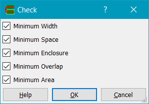
Displays the Check dialog. Width and spacing error checks can be performed if layer minWidth and minSpace properties have been set in the techfile or via loading LEF.
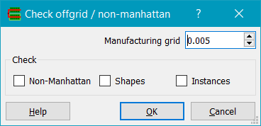
Displays the Check Offgrid dialog. If Non-Manhattan is checked, it will check and select any paths or polygons that contain non-manhattan edges. If Shapes is checked, it will check if any shape vertices are not on the specified Manufacturing grid. If Instances is checked, it will check if instance origins are on grid, and in the case of arrays that the rowSpacing and columnSpacing values are an integer multiple of the manufacturing grid. The command works on the top level cell only currently.
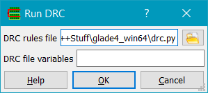
Shows the Run DRC dialog. Choose a DRC file and run DRC. Any existing DRC violation markers are erased. If an environment variable GLADE_DRC_FILE is set, the DRC rules file will be set to the value of GLADE_DRC_FILE (which must be a full path name). DRC file variables can be set using the DRC file variables entry; both the name and value are passed to Python as strings. Options should be in the form of name=value, separated by a space. If an environment variable GLADE_DRC_VARS is set, the variables will be set to the value of this env var.
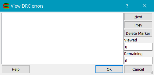
Steps through DRC errors. Click on a rule violation in the left hand list box to select the type of violation you wish to view. The first violation marker will be selected and zoomed in on. Subsequently you can use the Next and Prev buttons to step through the list of violation markers, zooming in on each new marker. The Delete Marker button will delete the currently viewed error marker. Viewed is the number of violations viewed so far; Remaining is the total number of violations remaining (the starting number less the number deleted using Delete Marker).
Clears all errors on the drcMarker layer.
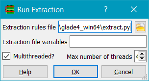
Shows the Run Extract dialog. Choose an extraction file and run extraction. If an environment variable GLADE_EXT_FILE is set, the extraction rules file will be set to the value of GLADE_EXT_FILE (which must be a full path name). Extrction file variables can be set using the Extraction file options entry. Options should be in the form of name=value, seperated by a space; both the name and value arepassed to Python as strings. Multithreaded if checked runs connectivity analysis in the number of threads specified in Max number of threads, which defaults to the maximum number of logical cores the machine can use. If an environment variable GLADE_EXT_VARS is set, the variables will be set to the value of this env var.
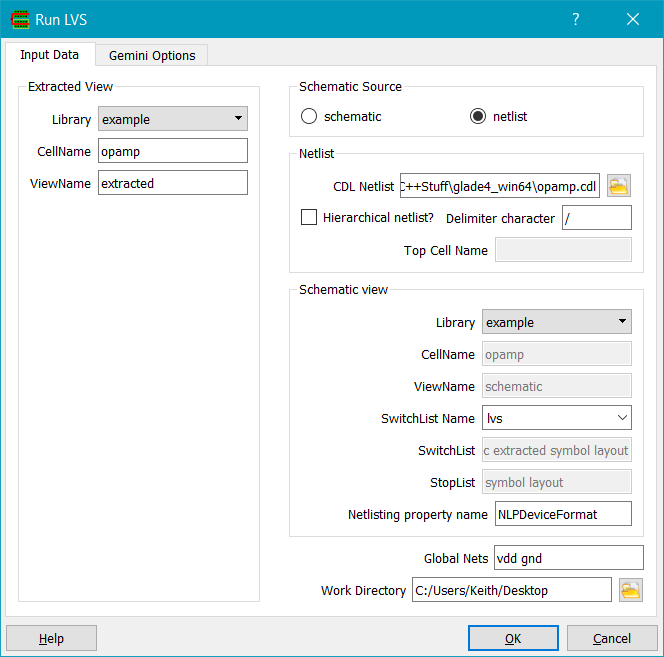
Shows the Run LVS dialog. Open an extracted view or specify the
name of an existing extracted view in the Library/CellName/ViewName fields.
If Schematic source is set to netlist, specify the name of the netlist in the CDL Netlist field. This can be preset via an enrionment
variable GLADE_NETLIST_FILE. If the Schematic source is set to schematic, the Schematic view panel is enabled and you can specify a library/cell/view name that will be netlisted and flattenned automatically.
Global Nets specifies global nets for the CDL netlist file. For a hierarchical netlist from a schematic, the Switch List and Stop List control the netlist hierarchy traversal. Switch/Stop/Globals lists are stored with a name tag, so multiple different switch/stop lists can be chosen from. The SwitchList name field is the name of the tag. You can edit this name to create a new tag, and the name and the switch/stop/globals lists will be stored in the gladerc.xml file so they can be recalled in future sessions. The Switch List is a list of view names that the netlister can descend into. The Stop List is a list of views that the netlister will stop descending into, and instead write the device to the netlist according to its NLPDeviceFormat property. If Hierarchical netlist? is checked, then a hierarchical netlist will be
flattened before passing to the LVS engine. Delimiter character
specifies the delimiter between hierarchical names of nets and instances.
Top Cell Name must be specified for
a hierarchical netlist; it is the top level .subckt name that corresponds to the
design to be verified.
The netlister property name can be set in the Netlisting property name field. It is a space-delimited list of names of the property to be used for netlisting; the first found is used, else the property name 'NLPDeviceFormat' is used.
Working Directory specifies a directory where temporary files are written. The
extracted view is netlisted to a CDL file which is compared to the specified
schematic netlist. Match info and/or discrepancies are written to the log
file. The
Gemini Options tab allows specification of Gemini options. 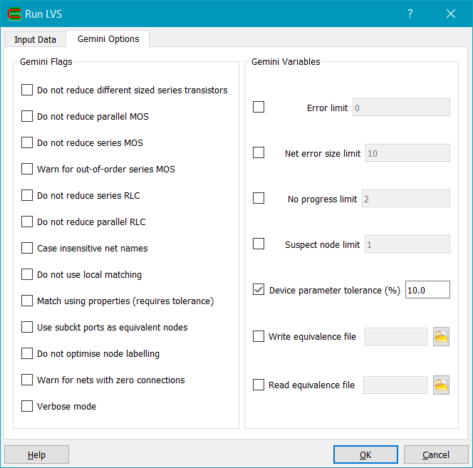
Gemini will write mismatch information to the message window, and to the open extracted view as error markers for nets/devices.
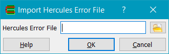
Imports a Hercules error file. The DRC error viewer can then be used to step through the errors.
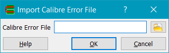
Imports a Calibre error file. The DRC error viewer can then be used to step through the errors. Both flat and hierarchical Calibre error files are supported.
Allows comparison of layers from two different cellviews using a multithreaded XOR operation. This can be useful for checking the changes made between two different versions of a design.
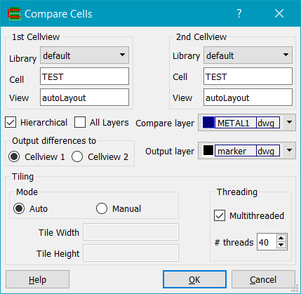
The data to be compared is specified by the 1st CellView and 2nd CellView. They are compared by the Compare layer using an XOR. If Hierarchical is checked, the cells are flattened for the compare, else only shapes on the Compare layer at the top level will be compared. If All Layers is checked, all the layers are compared, else just the Compare Layer .The results are output to the cellView specified in the Output differences to field. Results are written to the Output layer specified - if drcMarker is used (the default), then differences can be viewed using the DRC->View Errors command.
Comparison is done by multithreaded tiling of the original data to handle large designs. For setting tile sizes and multithreading options, see the Tiled Boolean Operations command.
Note: if you want to compare two cells by importing e.g. GDS2 or OASIS files, you MUST use import a techfile for each import with the same GDS layer/datatype to layer/purpose mapping. Failing to do this (e.g. importing two GDS2 files without importing any techfile) will most likely result in the GDS layer/datatype of one file being assigned to a different internal layer number from that of the second file. This is because internal layer numbers represent layer/datatype or layer/purpose pairs as a single number, and the mapping is assigned in the order the pairs are encountered.
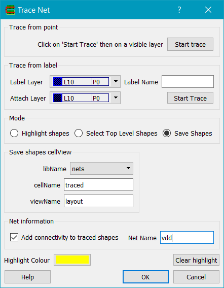
Traces connectivity either from a start point or from a text label. To use the net tracer, the technology file must have layers with their CONNECT attributes defined. For example:
   CONNECT poly drawing BY contact drawing TO metal1 drawing ;
	CONNECT metal1 drawing BY via1 drawing TO metal2 drawing ;
	CONNECT metal1 drawing TO metal1 drawing
In the first two cases, connection of the poly layer to the metal1 layer is through a via layer. In the second case, the two layers connect without any via layer.
To use the net tracer to trace from a shape, click on the Trace from point/Start Trace button. Tracing will continue until no more connecting shapes are found. Tracing may be aborted by clicking on the red abort button next to the progress bar on the status bar.
To use the net tracer to trace from a text label, set the Label Layer and the Attach Layer (which can be the same layer). Enter the Label Name and click on Trace from label/Start Trace . Note that currently, only labels on the top level of the cellView hierarchy can be traced from.
Mode selects whether traced shapes are highlighted (the default) or selected. Only shapes on the top level (currently displayed) cellView can be selected. The third option, 'Save Shapes', writes all traced shapes to a cellview, given by libName/cellName/viewName.
If the checkbox Add connectivity to traced shapes is set, then a net with the name given by Net Name will be created it it does not already exist, and all traced shapes will be assigned to that net. NB entering a Label name for tracing from a text label will automatically set the Net Name field.Clicking on Highlight Colour will alllow changing the highlight colour. Clear highlight clears all highlighted shapes. Using the selection options dialog to dim unhilited objects can make the trace result clearer.
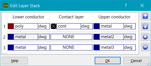
Displays the layer connectivity used for the Trace Net
command (and also settable in the techfile as described above, or
set during import of LEF/DEF). The dialog displays lower conducting layers,
optional contact layers and upper conduction layers. So in the above dialog,
poly connects to cont which connects to metal2. metal2 connects to metal, and
metal also connects to metal3.
To edit a layer, double click
on it and the icon will change to a combo box as shown in the second column,
third row of the dialog above. You can set the layer to any layer including a special
layer 'NONE' which when used for the contact layer means there is no explicit
contact layer between the conducting layers.
To add a row of connecting layers,
use the '+' buttton. To delete a row of layers, select the row by single
clicking on it, then use the '-' button. To move a row of layers up, select a
row and use the 'up' bottom. Similarly to move a row down, select the row and
use the 'down' button.
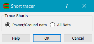
The Short Tracer can be used for DEF or similar designs that have connectivity. Either Power/Ground nets, or All Nets can be checked for touch/overlap against shapes connected to a different net. The bounding box of the shorting region is reported, and this bounding box is written to the drcMarker layer so that the DRC->View Errors dialog can be used to step through the errors, zooming to each short location. Currently only top level nets are checked against other top level nets; in other words the check is done flat.
Copyright © Peardrop Design 2026.